OBIEE 11g introduced several features in Action Frame Work that makes it possible to link BI content to several other content types via action links. One of the most common uses of action links is to setup drilldowns to other BI content. This a fairly straight forward process. In master analysis you need to include all columns that are defined as prompts. You can then setup action link in master report column properties to navigate to detail analysis. This is very easy to setup as long as both master and detail analysis are using same subject area.

What will happen if master and detail analysis are not coming from same subject area. It should work seamlessly as long as columns are same. I haven’t tried how it will behave if column names are same but coming from different business models. It would make a nice topic for another post.

In certain cases you may simply have no choice but to drilldown to detail report using URL. It could be due to different column names, or different business models or having the need to pass non-equi conditions or apply formula’s on column before they are passed.

For this post, I would like focus on how to dynamically construct a GO URL to drilldown report.

Dynamic URL for drilldown:

Below are two possible solutions.

Option 1:

Embedding HTML link in report column. Several bloggers have already explained this technique. You can find one good article from Cap Gemini BICG here

You can construct a GO URL to drilldown report with parameters and use that URL as hyperlink in master report using above technique. You can find an example of GO URL syntax here

You would have to manually change server name in URL when code is migrated to qa or prod from dev.

You can overcome this challenge by introducing a repository or session variable in RPD that has name of the server.

This is a tried and proven method by OBIEE developers for several years.

 

Option 2:

We can achieve similar result using action frame work “Invoke Browser Script” method. This option doesn’t require changing column format to HTML etc. However, you do need to know little bit about JavaScript.

In below example I have setup a master analysis and detail analysis. When I click on a product in master report it shows up in detail report. I’m being lazy to setup a complex scenario. This concept would work for any scenario.

 

Step 1:

Setup a javascript function that handles URL creation and calling in userScript.js

Every function you like to add to userScript.js has two entries in file. One for function definition and other for publishing it’s parameters to action frame work.

Notice my URL base. It starts with ‘saw.dll’. There is no need to worry about code migration from dev to qa to prod. It will automatically call corresponding objects from where ever you are running the code.

 

USERSCRIPT.navmyURL = function(aParams)

{

 

 

var urlbase = ‘saw.dll?PortalGo&path=%2Fshared%2FVenu%20Sample%2FURL%20parms%20Drill&Action=Navigate&col1=%22Products%22.%22Product%22&val1=’;

 

// sample URL http://t00764440:9704/analytics/saw.dll?PortalGo&path=%2Fshared%2FVenu%20Sample%2FURL%20parms%20Drill&Action=Navigate&col1=%22Products%22.%22Product%22&val1=13

 

 

var url = urlbase + aParams[‘pProdnum’];

 

 

window.open(url, “mywindow”);

 

};

 

USERSCRIPT.navmyURL.publish =

{

// The existence of this ‘publish’ object causes the ‘USERSCRIPT.example_displayParameters’ function to be

// shown when browing the available user script functions (during creation of a Script action).

 

// If you wish the Script function to have parameters automatically created on selection of the function,

// create a ‘parameters’ object as shown below.

// You can have any number of parameters, with each parameter requiring a unique name, prompt and an

// optional value.

 

//pProdnum

parameters :

[

new USERSCRIPT.parameter( ‘pProdnum’, ‘Enter value for Product Number’, ‘this will be set to the url’ )

]

 

// If no generated parameters are required, either create an empty array

// parameters : []

// or don’t declare the ‘parameters’ object at all.

};

 

Step2:

Once a function is defined in userScrip.js file, it will become available via Action Framework browser scripts option. I have defined product number as parameter to my function.

 

 

Step 3

 

Step 4:

People who are familiar with passing multiple parameter values to drill down reports using the GO-URL can now take a breath of fresh air.
In OBIEE 11g this is an in-built feature that obiee takes care of on deciding what parameters/columns are passed down to the sub report.

In order experience this feature we would first be creating a sub-report with two “is-prompted” prompts then secondly create a master/main report which will call the sub-report by passing the values to these two prompts.

1. The first sub-report creation is per below steps:
2. Go to your web analytics page: http://localhost:9704/analyticsand login using your username and password.
3. On the OBIEE Menu select New->Analysis->Select Subject Area->Sample Sales.
4. On the left Subject Area screen select the four columns and drag it to the right “Selected Columns” area as below:
   
5. Click the “Save Analysis” Icon at the top-right and enter “SubGOReport” under “Shared Folders”, “Sample Sales” directory as shown below:
6. Select the “Per Name Year” column options and select “Filter” and for the “Operator” select “is prompted” and click OK button.
7. Select the “Sales Rep Name” column options and select the “Filter” and for the “Operator select “is prompted” and click OK button.
8. Verify with screenshots as shown below:

   

   haeajgfb

   

   hajfeggh

9. Now we go on to creating the prompts for the above created filters.
10. Select the “Prompts” tab and then click the ” + ” , then select the “Column Prompt”, then the “Time”.”Per Name Year”.
11. When the “New Prompt” windows open make sure the below Operator and all the checkboxes are checked as below:
12. Click the ” + ” icon again, then select the “Column Prompt”, then the “Sales Rep”.”Sales Rep Name”.
13. When the “New Prompt” windows open make sure the below Operator and all the checkboxes are checked are as below:
14. After the two prompts have been created, click the “Save Analysis” icon to save the analysis and verify with below screenshot:
15. Click the “Results” tab and click on the “Show how results will look on a Dashboard” link, to make sure that your report is working.
16. Now we are done creating the Sub-report.
17. Now on to creating the second Main report which will call the sub-report.
18. Select New->Analysis->Select Subject Area->Sample Sales. to create a new report with the 3 columns as show below:
19. Click the “Save Analysis” icon to save your analysis with the name “MainGOReport” as show below:
20. Select “Revenue” column options, then “column properties” top open the “Column Properties” window.
21. Select the “Interaction” tab and then click the ” + ” icon to add “Add Action Link”.
22. When the “New Action Link …” window opens, click on the “Create New Action” icon and select “Navigate to BI Content”.
23. When the “Select BI Content For Action” window opens, go down to the “Shared Folders”, “Sample Sales” folder and select the “SubGOReport”.
24. Then click the OK button on all the 3 open windows to show your action links as below:
25. Click on the “OK” button to close the “Column Properties”.
26. Then click on the “Save Analysis” button to save your analysis.
27. Now click the “Results” Tab to see your report.
28. You can observe that the “Revenue” column now shows as links.
29. When you click on the dollar amount next to “Helen Mayes” in the Year “2008” you will see a Pop-Up showing you an option “SubGOReport”.
30. Click on the “SubGOReport”
31. Click OK button when asked to navigate away from this page:
32. Now should be able to see your “SubGOReport” report and “2008” selected for “Per New Year” prompt and “Helen Mayes” selected for “Sales Rep Name” prompt.

Summary:
From this exercise you can observe that the MainGOReport’s “Per Name Year” and “Sales Rep Name” values were sent down to the SubGOReport’s prompts and this
option can be used instead of the GO-URL option that was used earlier versions of OBIEE.

One of the welcome (but strangely unheralded) new features introduced with OBIEE 11.1.1.5 is support for Oracle OLAP as a data source. Earlier releases of OBIEE supported Oracle OLAP through SQL access, either directly through SQL views or through cube-organized materialized views, and there was even a plug-in to Analytic Workspace Manager to help you create the required repository metadata. This new release simplifies the process considerably though as the BI Administration tool can now connect directly to the Analytic Workspace metadata within an Oracle database, and allow you to import the cubes, dimensions, measures and other metadata from Oracle OLAP directly into the repository, in the same way that you do for an Essbase database. So how does this new support work?

According to the Oracle BI 11.1.1.5 Certification Matrix, Oracle OLAP 10.2, 11.1 and 11.2 are all supported as data sources. No specific patch levels are mentioned, but in general with Oracle OLAP you should always be on the latest patch release as critical updates are often made available through metalink even between major database releases. That said, for this example I’ve used the standard, unpatched version of Oracle OLAP that comes with Oracle Database 11.2.0.1, along with Analytic Workspace Manager 11.2.0.1.0 downloaded from OTN.

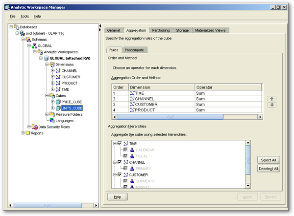
For the example I’ll be working with the Global sample OLAP dataset that’s also available from OTN, which in Analytic Workspace Manager looks like this:

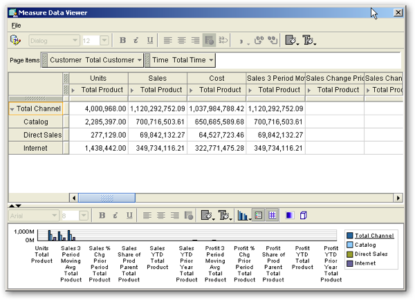
This dataset contains two cubes, which join to either all or a subset of the dimensions within the analytic workspace. There’s also some derived measures in the cubes, and all of the data has been processed and pre-aggregated, so that when viewed in Analytic Workspace Manager it looks like this:

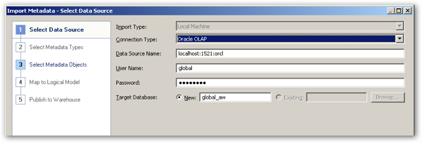
To import the metadata for this Oracle OLAP analytic workspace into an Oracle BI Repository, make sure you are using OBIEE 11.1.1.5 and start the Oracle BI Administration tool from the Windows Start Menu. Either open an existing repository online, or create a new one offline, and select Oracle OLAP as the data source. Then, enter the following details to connect to the database and view the list of analytic workspaces:

Connection Type : Oracle OLAP
Data Source Name : host:port:sid, e.g. localhost:1521:orcl
User Name : Username of account containing the analytic workspace, e.g. global
Password : Password for the above account
Target Database : Name for imported physical database in RPD physical layer, or name of existing physical database

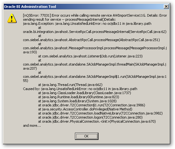
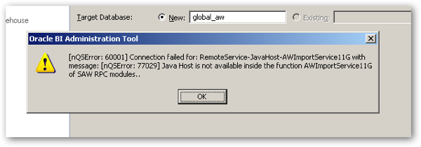
There’s a potential couple of “gotchas” here. Firstly, don’t type in a TNSNAMES entry (for example, “orcl”) as the Data Source Name, as you’ll get the following error if you do:

This error happens because the Administration Tool uses a new AWImportService java class to access the Analytic Workspace metadata, and it only takes connection details in the JDBC format (you can switch back to a TNSNAMES entry later in the process). If you hit this error, re-enter the connection details in the host:port:sid format and it’ll work.

The other error you might hit is if Javahost isn’t running when you try to make the connection.

This is because the Administration Tool uses Javahost (the system component that provides the ability for the C-based OBIEE components to run Java processes) to access AWImportService, even if you’re opening the repository offline. If this happens, make sure Javahost is running and it’ll then work, but this does then suggest that you need to perform this import on a server or workstation where OBIEE 11.1.1.5 is installed and running, otherwise the Administration Tool won’t be able to access a Javahost instance.

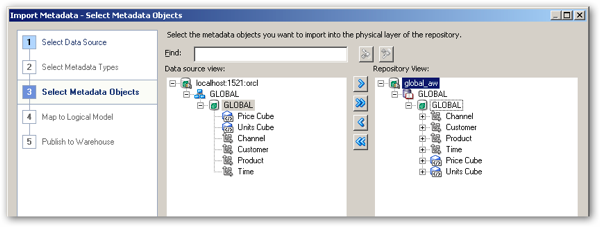
Once you connect, you’re presented with a list of all the analytic workspaces accessible to the account you connected with, which you can then select for import into the repository. Where this differs to importing Analytic Workspace-based views in OBIEE 10g is that you are also importing the hierarchies into the repository, as you do with an Essbase, SAP B/W or Microsoft Analysis Services metadata import.

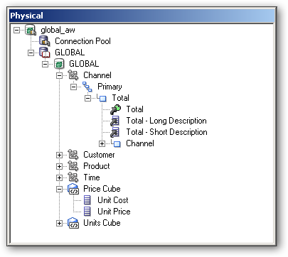
Once the import completes, you can see the physical database, Analytic Workspace, Oracle OLAP dimensions, hierarchies, cubes and measures that you’ve imported, in the Physical layer of your repository.

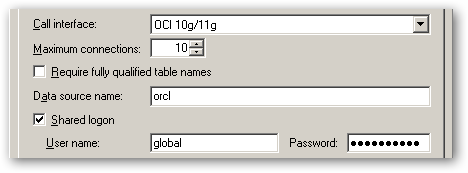
Before you can access data from the analytic workspace through the repository, you’ve got to make a quick change in the connection pool connection details to go back to a TNSNAMES entry. Double-click on Connection Pool within the new database and edit the Data source name entry so that it uses a TNSNAMES entry rather than the host:port:sid that’s there because of the previous step.

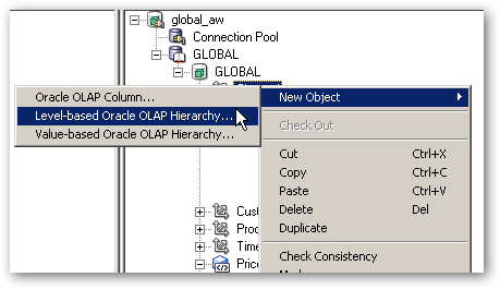
Looking inside the Physical layer metadata that’s been created using the Import Wizard, you can see that hierarchies within an Oracle OLAP dimension can be either level-based, or parent-child. This is the same as with Essbase physical hierarchies, although from an initial test it doesn’t look like you can alter an already-imported hierarchy from one type to the other, meaning that you’ll only be able to switch from level-based to value-based hierarchies if you change the underlying hierarchy type in the analytic workspace itself.

This could potentially be an issue as, like with Essbase sources, it doesn’t appear you can “re-import” an analytic workspace definition back into the repository to pick up new hierarchy levels. It’s early days yet though but, as with Essbase sources, if you’re testing this out, bear in mind that the analytic workspace definition may change over time, and you’ll need to work out how to reflect those changes in your repository without breaking all the existing mappings and analyses.

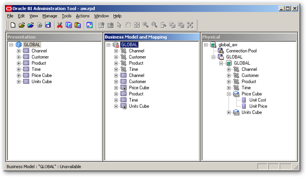
So once you’ve imported the analytic workspace metadata into the physical layer of the repository, as with an Essbase database, you can then drag and drop the cube definition first into the Business Model and Mapping Layer, and then the Presentation Layer, of your repository, so that it looks like this:

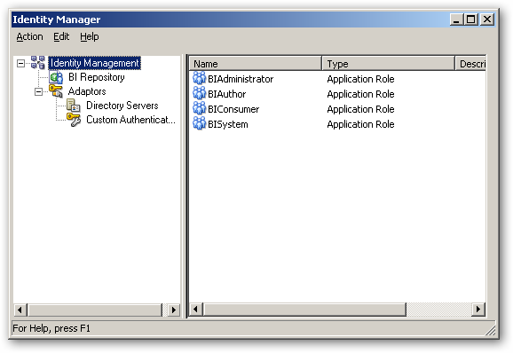
Now the various layers of the repository metadata are complete, I upload the RPD file to the Oracle BI Instance ready to run my first analysis. Before I do this though, I enable query logging at level 5, so that I can see the physical SQL, and the logical execution plan, for the analyses I create. With the Oracle BI repository online now, I select Manage > Identity from the BI Administration application menu, and notice that, even though I’m connected to an online repository, whilst my application roles are listed, there are no users.

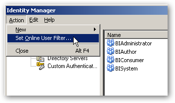
So what’s going on here then? Well, in 11.1.1.5, there’s an enhancement with the Identity Manager dialog where, by default, users from the LDAP server are filtered so that WebLogic doesn’t try and return all LDAP users every time you open this dialog. To change this filter (which by default is set to blank, and has to be set to “*” to return all users), select Action > Set Online User Filter from the Security Manager dialog and then enter the search filter.

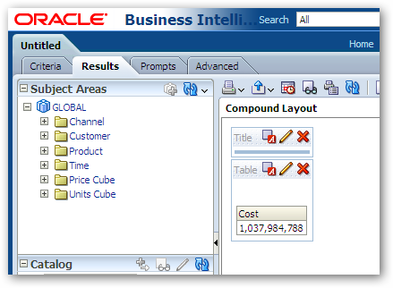
So now with logging set to level 5 for the weblogic user, I use my web browser to bring up the Oracle BI homepage and run a simple query to return the total for costs across all dimensions.

So what does the SQL look like, that the BI Server has generated to return this result? I take a look at the NQQuery.log file and find the entry for this analysis.

WITH
SAWITH0 AS (select distinct case when count(*) > 1 then null else max(units_cube_cost) end as c1
from
(select *
from table(olap_table('GLOBAL.GLOBAL duration session', '', '',
'measure units_cube_cost from UNITS_CUBE_COST ' ||
'dimension channel_id as varchar2(100) from CHANNEL with ' ||
'  attribute channel_level as varchar2(100) from CHANNEL_LEVELREL ' ||
'  hierarchy CHANNEL_PARENTREL(CHANNEL_HIERLIST ''PRIMARY'') ' ||
'    inhierarchy CHANNEL_INHIER ' ||
'dimension customer_id as varchar2(100) from CUSTOMER with ' ||
'  attribute customer_level as varchar2(100) from CUSTOMER_LEVELREL ' ||
'  hierarchy CUSTOMER_PARENTREL(CUSTOMER_HIERLIST ''SHIPMENTS'') ' ||
'    inhierarchy CUSTOMER_INHIER ' ||
'dimension product_id as varchar2(100) from PRODUCT with ' ||
'  attribute product_level as varchar2(100) from PRODUCT_LEVELREL ' ||
'  hierarchy PRODUCT_PARENTREL(PRODUCT_HIERLIST ''PRIMARY'') ' ||
'    inhierarchy PRODUCT_INHIER ' ||
'dimension time_id as varchar2(100) from TIME with ' ||
'  attribute time_level as varchar2(100) from TIME_LEVELREL ' ||
'  hierarchy TIME_PARENTREL(TIME_HIERLIST ''CALENDAR'') ' ||
'    inhierarchy TIME_INHIER ' ||
'loop optimized ' ||
'row2cell r2c '
))
where channel_level = 'TOTAL' and customer_level = 'TOTAL' and product_level = 'TOTAL' and time_level = 'TOTAL' and (units_cube_cost is not null)
))
select distinct 0 as c1,
D1.c1 as c2
from
SAWITH0 D1

So what’s different here, compared to previous support for Oracle OLAP, is that the BI Server is writing the query using the OLAP_TABLE function, rather than accessing AW objects via SQL views, and it’s using 11g features such as “loop optimized” that Stewart covered in this earlier blog post on new capabilities in Oracle OLAP 11g. Notice also that the OLAP_TABLE function references all dimensions associated with the measure (albeit at “TOTAL” level) even though they’re not included in the analysis, as that’s the way that OLAP_TABLE works.

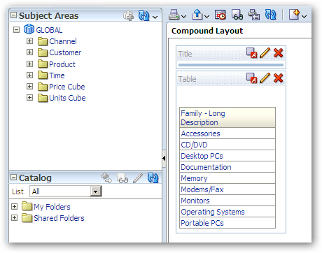
Next I run another simple query, this time just accessing an attribute from the product dimension.

This time, as I’m only accessing a dimension and note a measure, the OLAP_TABLE function just references the dimension in the function clause.

WITH
SAWITH0 AS (select distinct family_product_long_descripti1 as c1
from
(select *
from table(olap_table('GLOBAL.GLOBAL duration session', '', '',
'dimension product_id as varchar2(100) from PRODUCT with ' ||
'  attribute product_level as varchar2(100) from PRODUCT_LEVELREL ' ||
'  hierarchy PRODUCT_PARENTREL(PRODUCT_HIERLIST ''PRIMARY'') ' ||
'    inhierarchy PRODUCT_INHIER ' ||
'    familyrel family_product_long_descripti1 as varchar2(100) from ' ||
'      PRODUCT_FAMILYREL(PRODUCT_LEVELLIST ''FAMILY'') ' ||
'      label PRODUCT_LONG_DESCRIPTION ' ||
'row2cell r2c '
))
where product_level = 'FAMILY'
))
select distinct 0 as c1,
D1.c1 as c2
from
SAWITH0 D1
order by c2

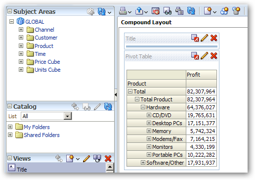
So what about using a hierarchical column? As a quick reminder, when you use a a hierarchical column within OBIEE 11g, the Presentation Server sends a request to the BI Server, which then generates logical requests for each subtotal within the hierarchy. For relational sources, the BI Server then joins these logical queries together into a single (rather large) physical SQL request using subquery factoring (subqueries and WITH clauses). With Essbase (and other MDX-based) sources though the BI Server can’t do this, and instead fires of lots of individual MDX queries to the Essbase server, and then joins the resultsets together again before passing the results back to the Presentation Server. This can cause quite an excessive load on the Essbase server, so I’m keen to see how this works with Oracle OLAP.

To start off, I create a simple analysis where I drill into the product dimension, and display it along with one of the measures in the analytic workspace, like this:

Taking a look at the logical execution plan and resulting physical SQL that this generates, the BI Server has indeed generated multiple logical SQL queries (as it would with relational sources), but unlike an Essbase source the resulting physical SQL is all in a single query. So in some senses OBIEE 11g queries against Oracle OLAP sources are more efficient than Essbase ones, as the BI Server is able to keep the hierarchical column query as a single SQL statement rather than generating lots of MDX statements as it does with MDX-based sources.

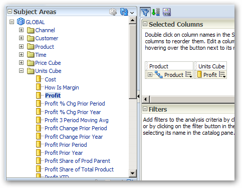
Another nice feature of Oracle OLAP is that it’s very easy, using Analytic Workspace Manager, to derive time-series measures based off of a set of base measures. In the Oracle OLAP cube that we’ve imported in, you can see these under the presentation fact table, and these can be selected like any other measure to add to your analysis criteria.

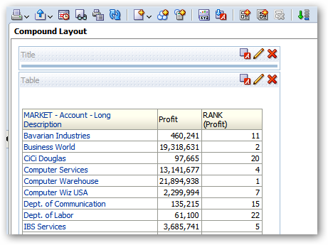
So one last test I’d like to do, because this is a weak area of the way that Essbase is integrated into OBIEE, is around function push-down. For Essbase and other MDX-based OLAP sources, very few OBIEE functions are shipped-down to their corresponding MDX functions, which can affect performance as the BI Server has to provide ranking and other such calculations for Essbase sources, even though they’re more than capable of doing this themselves. So let’s try a rank function in an analysis and see what happens.

So how does the SQL look?

WITH
SAWITH0 AS (select case when count(*) > 1 then null else max(units_cube_profit) end as c1,
account_customer_long_descrip1 as c2,
account_customer as c3
from
(select *
from table(olap_table('GLOBAL.GLOBAL duration session', '', '',
'measure units_cube_profit from UNITS_CUBE_PROFIT ' ||
'dimension channel_id as varchar2(100) from CHANNEL with ' ||
'  attribute channel_level as varchar2(100) from CHANNEL_LEVELREL ' ||
'  hierarchy CHANNEL_PARENTREL(CHANNEL_HIERLIST ''PRIMARY'') ' ||
'    inhierarchy CHANNEL_INHIER ' ||
'dimension customer_id as varchar2(100) from CUSTOMER with ' ||
'  attribute customer_level as varchar2(100) from CUSTOMER_LEVELREL ' ||
'  hierarchy CUSTOMER_PARENTREL(CUSTOMER_HIERLIST ''MARKET'') ' ||
'    inhierarchy CUSTOMER_INHIER ' ||
'    familyrel account_customer as varchar2(100) from ' ||
'      CUSTOMER_FAMILYREL(CUSTOMER_LEVELLIST ''ACCOUNT'') ' ||
'      label CUSTOMER ' ||
'    familyrel account_customer_long_descrip1 as varchar2(100) from ' ||
'      CUSTOMER_FAMILYREL(CUSTOMER_LEVELLIST ''ACCOUNT'') ' ||
'      label CUSTOMER_LONG_DESCRIPTION ' ||
'dimension product_id as varchar2(100) from PRODUCT with ' ||
'  attribute product_level as varchar2(100) from PRODUCT_LEVELREL ' ||
'  hierarchy PRODUCT_PARENTREL(PRODUCT_HIERLIST ''PRIMARY'') ' ||
'    inhierarchy PRODUCT_INHIER ' ||
'dimension time_id as varchar2(100) from TIME with ' ||
'  attribute time_level as varchar2(100) from TIME_LEVELREL ' ||
'  hierarchy TIME_PARENTREL(TIME_HIERLIST ''CALENDAR'') ' ||
'    inhierarchy TIME_INHIER ' ||
'loop optimized ' ||
'row2cell r2c '
))
where channel_level = 'TOTAL' and customer_level = 'ACCOUNT' and product_level = 'TOTAL' and time_level = 'TOTAL' and (units_cube_profit is not null)
)
where  ( 1 = 1 )
group by account_customer_long_descrip1, account_customer),
SAWITH1 AS (select distinct 0 as c1,
D1.c2 as c2,
D1.c1 as c3,
Case when D1.c1 is not null then Rank() OVER ( ORDER BY D1.c1 DESC NULLS LAST ) end as c4,
D1.c3 as c5
from
SAWITH0 D1)
select D1.c1 as c1,
D1.c2 as c2,
D1.c3 as c3,
D1.c4 as c4
from
SAWITH1 D1
order by c1, c2

Well, whilst the RANK() calculation hasn’t been converted to OLAP DML and performed by the analytic workspace, it has been performed by the database rather than having to be done by the BI Server. In a way it’s academic as by the time the numbers have been summed up, ranking them is a much simpler job, but it looks like aggregate and other analytic functions pushed-down by the BI Server will get added to the Oracle SQL statement that summarizes the results of the OLAP_TABLE query.

So, dare I say it, it looks like proper Oracle OLAP support in OBIEE 11.1.1.5 works pretty well, at least based on first impressions. It doesn’t suffer from the same “square peg in a round hole” syndrome that you get when the BI Server tries to convert from relational SQL to multidimensional MDX, because it’s the Oracle Database that does this conversion, through the OLAP_TABLE function. Of course, with all new features and in particular, new data source support, the “devil is in the detail”, but it’s certainly an encouraging start. If anyone implements Oracle OLAP through this new approach, I’d be interested to hear how you get on.